
How many television shows have you seen where the hunter describes how they “patterned” the deer they shot? They knew the deer was going to be there because of the scouting they had done. How many magazine articles have you read where the author describes how they had learned the habits of a particular deer by watching him for several years? Of course, their attention to detail and commitment to understanding their quarry enabled them to succeed where so many have failed.
The reality is that individual deer are extremely difficult to pattern, if not impossible. Good hunters use their knowledge of the biology of deer to identify locations where there is a good probability of seeing bucks. Great hunters use their knowledge of the biology of deer to identify locations where there is a good probability of seeing mature bucks. Story tellers describe to you how they used their skills as a woodsman to learn the habits of a deer they had been watching for several years, and how they applied their knowledge of his habits to outsmart him.
A lot can be learned from the spatial patterns (daily and seasonal movements) of white-tailed deer, and understanding their patterns can undoubtedly improve our effectiveness as hunters and/or managers. However, a few glimpses of a deer in the woods, combined with a few pictures from game cams, does not begin to describe the spatial pattern of a deer, much less enable a hunter to predict where a specific deer will travel. A more scientific approach is required to develop an understanding of the spatial ecology of white-tailed deer, but even highly technological approaches will not predict where an individual deer will move to next.
There are three aspects of the spatial patterns of deer that should be of particular interest to hunters and managers. An understanding of these patterns should improve a hunter’s knowledge of buck movements during the breeding season, which should translate into improved hunting success. First, bucks display particular characteristics of movement during 24-hour periods, which I would describe as primary movements. Second, the sum of all primary movements (secondary movement pattern) during the breeding season defines the home range of a deer. The third aspect of the spatial ecology of bucks could be defined as tertiary patterns, and I would describe the tertiary pattern of deer movement as shifts in home range from year to year.
Herein I describe the results of a 3-year study on the movement patterns of mature male white-tailed deer during the breeding season. The population that we studied was comprised of more than 50% mature (3.5 years old or greater) males and was open to public hunting. We affixed radio collars to 80 bucks that ranged in age from 2.5 to 9.5 years, and collected data using radio telemetry.
Primary Movements
We located individual deer every 3 hours for a 24-hour period to try and develop an understanding of how bucks moved across the landscape during a typical day. We did this approximately 500 times during the 3 year period, and developed a pretty interesting data set, which is unique to the best of my knowledge.
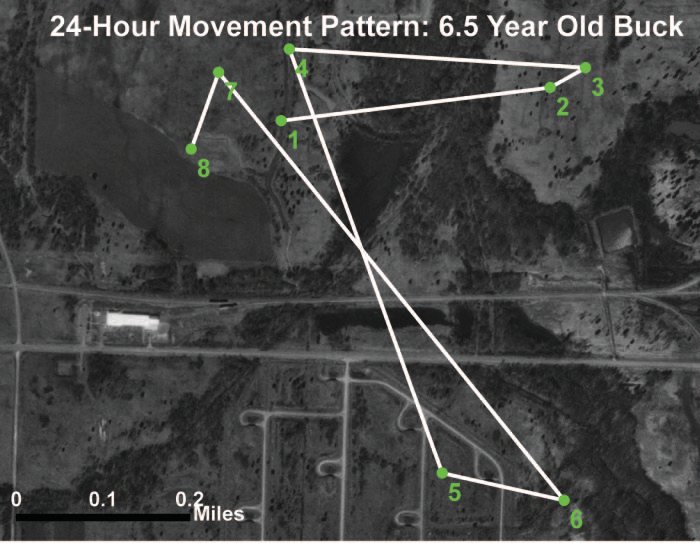
The standard movement pattern that we documented during the breeding season can be seen in Figure 1. Deer would move at least 3 miles on average during a 24-hour period (note that this estimate is the minimum distance moved, as the deer could have wandered considerably between consecutive locations), and as you can see, their movement track could almost be described as random as they repeatedly crossed their home range in search of does. Even after following these animals continuously, and doing this with some individuals over 25 times, it was still impossible to predict where that deer would move to next.
While collecting data, it became apparent that younger males frequently exhibited different patterns of movement than older males during a 24-hour period. Older males almost always followed the pattern shown in Figure 1. But, younger males (2.5 years old and younger) often displayed long, linear movement patterns during a 24-hour period. This can be seen in Figure 2. These young bucks would often begin moving in one direction, and continue moving in that direction for half a day, and then turn around and return during the next 12 hours. In Figure 2, you can see that the deer stayed in one general location for the majority of the day, and then began a long exploratory movement. We detected the beginnings of this movement between locations 7 and 8.

We hypothesize that these movements were exploratory, and were a response to the presence of a large number of more dominant, mature males in the population. While searching for does, we suspect that the younger males were continuously subjected to aggressive encounters with dominant bucks. As a result, they would occasionally venture on an exploratory movement to assess if breeding opportunities were greater in other areas.
In one case we found a young male that moved about 2 miles to another area during the breeding season, stayed there for approximately a week, and then returned to his original home range. But, this was the exception, as males normally did not stay any place other than their original home range for longer than a few hours. We suspect that they never located any areas with improved mate availability, as there was a high density of mature bucks across the entire study area.
The other general observation that was apparent was: bucks rarely stopped moving during the peak of the breeding season. Most people have heard that bucks move 20-22 hours per day during that period, and our observations support that notion.
Secondary Movements
Home range size of deer during our study was not dissimilar to home range sizes reported for male deer in other studies. The mean home range of deer in our study during the breeding season was 1,200 acres. This is on the high end for the Southeast, and may be a function of the lower deer density (30 deer/mile2) on our study area as opposed to what is commonly found in other areas of the region. As a landowner or manager, you need to understand what this means from a management perspective. In essence, when you see a deer or capture a deer with a game cam, you need to understand that he may be on the edge of his home range (or in the middle). Based upon what we found with our 24-hour data, and the propensity of bucks to traverse their entire home range during a single day, it is entirely possible that he will be over a mile away in a few hours.
Another noteworthy pattern that we detected was the lack of a consistent pattern of how an individual deer utilized his home range during the breeding season. During summer, we were very good at predicting the locations of individual bucks based upon where we had seen them before. Some bucks we could predict would be on a food plot in the afternoon, and our prediction would prove correct 50% of the time. Others could be found at specific locations as well, feeding on the same plant communities evening after evening. We had the ability with one particular mature deer to stop the truck at a specific corner, and see him 4 out of 5 evenings during the last hour of daylight: he was almost always within about 150 yards of that corner. If we didn’t see him immediately, we would climb into the bed of the truck for a better vantage, and often see him feeding in the surrounding brush. If we still couldn’t get a glimpse, we would grab the telemetry gear to make sure he wasn’t dead. More often than not he was right there, but just not visible.
These patterns were not apparent during the breeding season. At any particular time of the day, it was possible to locate a buck at any point in his home range. There was no tendency for an individual to use the same bedding area on consecutive days (although I am sure that they did use the same bedding areas more than once as these are creatures of habit), so it was impossible to predict that a specific deer may approach a feeding area down a particular trail. One evening they could be seen traveling along the edge of a hardwood drain. The next evening the same deer would be located in a thicket 1.5 miles away, only to be found across his home range area on an oak ridge where does could be found feeding on acorns. This same consistent lack of pattern was apparent in both immature and mature bucks.
Tertiary Movements
The final characteristic of deer spatial patterns can be defined as tertiary movements. These are the similarities (or lack of) in home ranges from season to season or year to year. We have the ability, without the use of fancy radio telemetry gear, to get an idea about the extent to which an individual buck ranges with the use of game cams. By carefully examining pictures from game cams, and sightings by hunters, we can form a rough estimate of the real estate that is used by a particular deer. This is good use of technology and an intelligent way in which to begin the task of outsmarting a buck. But, you should be aware of some of the pitfalls of this approach.
First, preseason scouting (game cams and visual observations) is a fantastic way to select the wrong area to hunt a specific deer. The bucks in our study frequently used different home ranges during the spring and summer than they did during the breeding season. In some cases, these home ranges could be separated by several miles. Thirty percent of our deer shifted their area of core use (area where they spend the majority of their time) by over half a mile between the breeding and non-breeding seasons. What this means is that some of the deer you are scouting on your land in August may be several miles (or at least a half mile) away come hunting season. In one case, we had a deer that would spend the spring and summer a distance of five miles from his breeding home range: this occurred during three consecutive years. So, if you pass up or miss a buck during the season, and you don’t see him on cameras during spring or summer, don’t fret. He may very well still be alive. Of course, deer on your property during the spring and summer may not be there during the breeding season.
The next aspect of our tertiary movements to consider is the difference in breeding season home ranges from season to season. On average, there was 53% overlap between a specific buck’s breeding season home range one year and that during the next. This pattern was very consistent from animal to animal and from year to year. You should expect these shifts in home range, and understand how they could influence your approach to hunting an animal that you had chased during a previous season. To put it simply, there is only a 50% chance that the buck will ever walk anywhere near a location you choose to hunt (if you are choosing your stand placement based upon last year’s knowledge).

Figure 3 provides a good example of the pattern, or lack of a pattern, that I am describing. In year 1, the deer had a home range of 900 acres. During year 2, the home range size of the deer was similar (1,047 acres), but only 435 acres (41.5%) of that range overlapped that of the first year. I hypothesize that these bucks are keying in on perceived availability of does, which is a function of availability of seasonal foods. More specific, in this case, the diversity of oak species and availability of acorns on the study area caused does to concentrate their feeding efforts in different areas each year, and this buck adjusted accordingly.
The take home message from this data set is: don’t fool yourself into thinking you know more than you do about the animal that you are pursuing. His patterns of movement are more complex than we give credit for, and this can be the downfall of a hunter who is overconfident in his or her preparation for the hunt. To me, this data set highlights the importance of understanding deer and deer movements, not the movements of a specific deer. Use your knowledge of deer and deer biology to put yourself in a position for success, and maybe you’ll see the deer you hope to see.